Lets practice Backpropagation
In the previous post we went through a system of nested nodes and analysed the update rules for the system.We also went through the intuitive notion of backpropagation and figured out that it is nothing but applying chain rule over and over again.Initially for this post I was looking to apply backpropagation to neural networks but then I felt some practice of chain rule in complex systems would not hurt.So,in this post we will apply backpropogation to systems with complex functions so that the reader gets comfortable with chain rule and its applications to complex systems.
Lets get started!!!
Lets start with a single node system but this time with a complex function:
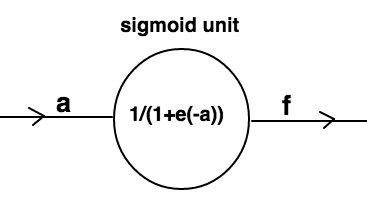
This system can be represented as:
import numpy as np
def sigmoid(x):
	return 1/(1+np.exp(-x))
a=-2
f=sigmoid(a)
print(f) #outputs 0.1192
Aim
Our aim essentially remains the same as in previous posts viz:we have to increase the value of output(f) by manipulating the values of input(a).
The node in above figure represents a sigmoid unit.Sigmoid function is expressed as- $$\Large\sigma({x})=\frac{1}{1+e^{-x}}$$
If you analyse the sigmoid function,you will notice that irrespective of the input value,this function gives a value between 0 and 1 as output.It is a nice property to have as it gives a sense of probabilistic values of inputs.It was once the most popular activation function used in neural network design.
Where do we start?Once again let us look at our update rule: $$\Large{a}={a}+{h}*\frac{df}{da}$$
(Here we are using total derivative(\(\Large{d}\)) instead of partial derivative(\(\Large\partial\)) because here our node is a function of only one variable i.e. a.And thats the only difference there is between the two notations.Rest everything remains the same.)
We just have to find value of the derivative \(\Large\frac{df}{da}\). If you are aware of basic rules of calculus(Refer Derivetive rules) then you can easily find the derivative of sigmoid with respect to a.If you are new to calculus then just remember for now that derivative of sigmoid funtion is given by:
$$\Large\frac{d\sigma}{da}=(\sigma({a}))*(1-\sigma({a}))$$
Let us put this value in our update rule: $$\Large{a}={a}+h*(\sigma({a}))*(1-\sigma({a}))$$
Using this update rule in python:
import numpy as np
def sigmoid(x):
	return 1/(1+np.exp(-x))
def derivative_sigmoid(x):
	return sigmoid(x)*(1-sigmoid(x))
a=-2
h=.1
a=a+h*derivative_sigmoid(a)
f=sigmoid(a)
print(f)  #outputs 0.1203
The above program outputs 0.1203 which is greater than 0.1192.It worked!!!
Let us take the discussion one notch above.Consider the system:
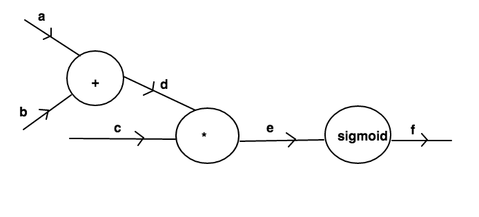 The system consists of three inputs
 a,b and c.The former two pass through an addition node and give output d which products with the inputc to generate e which is passed through sigmoid node to give final output f.Let us represent this system in python:
import numpy as np
def addition(x,y):
	return x+y
def product(x,y):
	return x*y
def sigmoid(x):
	return 1/(1+np.exp(-x))

a=1
b=-2
c=-3
d=addition(a,b)
e=product(c,d)
f=sigmoid(e)
print(f)  #outputs 0.952574
Our aim essentially remains the same viz:to tweak the values of input a,b and c in order to increase the value of f.Once again like our previous approaches,let us look at our update rules:
$$\Large{a}={a}+{h}*\frac{\partial f}{\partial a}$$ $$\Large{b}={b}+{h}*\frac{\partial f}{\partial b}$$ $$\Large{c}={c}+{h}*\frac{\partial f}{\partial c}$$
We have to somehow find the values of the derivatives \(\Large\frac{\partial f}{\partial a}\),\(\Large\frac{\partial f}{\partial b}\) and \(\Large\frac{\partial f}{\partial c}\).
Using chain rule described in previous post we can write: $$\Large\frac{\partial f}{\partial a}=\frac{\partial f}{\partial e}*\frac{\partial e}{\partial d}*\frac{\partial d}{\partial a}$$ $$\Large\frac{\partial f}{\partial b}=\frac{\partial f}{\partial e}*\frac{\partial e}{\partial d}*\frac{\partial d}{\partial b}$$ $$\Large\frac{\partial f}{\partial c}=\frac{\partial f}{\partial e}*\frac{\partial e}{\partial c}$$
This is a good example to get an intuition about chain rule.Observe how in order to compute derivatives of
fwith respect to various inputs,we are just travelling to those inputs fromfand multiplying(chaining) the derivatives that we encounter as we reach the input.
Lets start finding the values of derivatives:
Let us traverse the system from output to input i.e. backward.While crossing the sigmoid node the value of \(\Large\frac{\partial f}{\partial e}\) can be written easily as \(\Large(\sigma({e}))*(1-\sigma({e}))\).Further while crossing the product node the values of \(\Large\frac{\partial e}{\partial d}\) and \(\Large\frac{\partial e}{\partial c}\) can easily be written as \(\Large{c}\) and \(\Large{d}\) respectively.Further while crossing the addition node the values of \(\Large\frac{\partial e}{\partial d}\) and \(\Large\frac{\partial e}{\partial c}\) can be easily written as \({1}\) and \({1}\) respectively.If you are having trouble in getting your head around these derivatives,I suggest you to have a look at first and the second post of this series.
Writing our update rules we get: $$\Large\frac{\partial f}{\partial a}=(\sigma({e}))*(1-\sigma({e}))*{c}*{1}$$ $$\Large\frac{\partial f}{\partial b}=(\sigma({e}))*(1-\sigma({e}))*{c}*{1}$$ $$\Large\frac{\partial f}{\partial c}=(\sigma({e}))*(1-\sigma({e}))*{d}$$
Let us represent this in python:
import numpy as np
def addition(x,y):
	return x+y
def product(x,y):
	return x*y
def sigmoid(x):
	return 1/(1+np.exp(-x))
def derivative_sigmoid(x):
	return sigmoid(x)*(1-sigmoid(x))
#initialization
a=1
b=-2
c=-3
#forward-propogation
d=addition(a,b)
e=product(c,d)
#step size
h=0.1
#derivatives
derivative_f_wrt_e=derivative_sigmoid(e)
derivative_e_wrt_d=c
derivative_e_wrt_c=d
derivative_d_wrt_a=1
derivative_d_wrt_b=1
#backward-propogation (Chain rule)
derivative_f_wrt_a=derivative_f_wrt_e*derivative_e_wrt_d*derivative_d_wrt_a
derivative_f_wrt_b=derivative_f_wrt_e*derivative_e_wrt_d*derivative_d_wrt_b
derivative_f_wrt_c=derivative_f_wrt_e*derivative_e_wrt_c
#update-parameters
a=a+h*derivative_f_wrt_a
b=b+h*derivative_f_wrt_b
c=c+h*derivative_f_wrt_c
d=addition(a,b)
e=product(c,d)
f=sigmoid(e)
print(f)  #prints 0.9563
The output of above program is 0.9563 which is greater than 0.9525.
Similarly you can backpropagate through any complex system containing complex functions to generate update rules and thus manipulate the value of output by applying those update rules.
In the next post we will look to apply backpropagation to neural networks.We will start by a simple two layered network and then extend our discussion to three-layered network.
Posted on 16 January,2017