Into-Backpropagation

In the previous post,we learnt to appreciate the beauty of derivatives and their effect on update rule which is given by-

$$\Large{a}={a}+{h}*\frac{\partial f}{\partial a}$$ $$\Large{b}={b}+{h}*\frac{\partial f}{\partial b}$$

where $$\Large{f}={f}({a},{b})$$

Although the case of single node system helps us capture the intuition behind the effect of change in input on the output of node,it is pretty useless if considered in isolation.We need to scale up our network.Let us consider case of nested nodes as shown below-

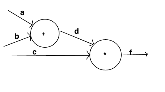
Here there are two nodes,out of which the first one(from the left) accepts two inputs a and b and performs addition operation on them to return the output d.The second node accepts d and a new input c as inputs and performs product operation on them to gives f as final output. This system can be represented in python:

def product(x,y):
	return x*y
def addition(x,y):
	return x+y

a=5
b=-3
c=-2
d=addition(a,b)
f=product(d,c)  #outputs -4

Aim

Our aim is still the same as was in last post viz;we want to manipulate the values of our inputs a,b,c in such a way that the value of output f increases.

Not only will we achieve the above aim but in that process we will slowly slide into backpropagation and go through the concept intuitively.Note that this post will be slightly more mathematical than the last one but all the concepts used are described intuitively in the previous post.

Lets get started!!

This nested system might seem a bit intimidating at first.Where do we start?Well,we know the update rules from the last post that involve derivatives of output with respect to input.Let us list down these update rules for our inputs a,b and c-

$$\Large{a}={a}+{h}*\frac{\partial f}{\partial a}$$ $$\Large{b}={b}+{h}*\frac{\partial f}{\partial b}$$ $$\Large{c}={c}+{h}*\frac{\partial f}{\partial c}$$

We somehow want to compute the three derivatives \(\Large\frac{\partial f}{\partial a}\),\(\Large\frac{\partial f}{\partial b}\) and \(\Large\frac{\partial f}{\partial c}\)

Let us look at the relations among various variables in our system.We can easily write-

$$\Large{f}={d}*{c}$$ $$\Large{d}={a}+{b}$$

Now let us use the analytical gradient to calculate derivatives from the above relations.(Refer Derivative rules).

Consider the relation \(\Large{f}={d}*{c}\)

Differentiating this relation we get-

$$\Large\frac{\partial f}{\partial d}={c}$$ $$\Large\frac{\partial f}{\partial c}={d}$$

Differentiating the relation \(\Large{d}={a}+{b}\) we get-

$$\Large\frac{\partial d}{\partial a}={1}$$ $$\Large\frac{\partial d}{\partial b}={1}$$

Observe that derivatives for addition node is 1.This makes intuitive sense too.If you try to increase input to an addition node by a quantity h,then the output value will increase by same quantity.Thus normalised change i.e. the derivative is 1.

We now have the values of \(\Large\frac{\partial f}{\partial d}\),\(\Large\frac{\partial f}{\partial c}\),\(\Large\frac{\partial d}{\partial a}\)and \(\Large\frac{\partial d}{\partial b}\).We somehow have to use these values to compute the values of \(\Large\frac{\partial f}{\partial a}\),\(\Large\frac{\partial f}{\partial b}\) and \(\Large\frac{\partial f}{\partial c}\).

The value of \(\Large\frac{\partial f}{\partial c}\) is already known.This leaves us with two unknown values viz:\(\Large\frac{\partial f}{\partial a}\) and \(\Large\frac{\partial f}{\partial b}\).

Backpropagation

Its time to introduce Chain rule.No need to be intimidated by the name.Its pretty easy and straightforward.We know the derivative of f with respect to d(\(\Large\frac{\partial f}{\partial d}\)) and we also know the derivative of d with respect to a(\(\Large\frac{\partial d}{\partial a}\)).Chain rule tells us how we can combine these two derivatives to find the derivative of f with respect to a( \(\Large\frac{\partial f}{\partial a}\)).It simply states to multiply these two derivatives(or to chain them together)to get the derivative of f with respect to a.Mathematically- $$\Large\frac{\partial f}{\partial a}=\frac{\partial f}{\partial d}{*}\frac{\partial d}{\partial a}$$

Similarly, $$\Large\frac{\partial f}{\partial b}=\frac{\partial f}{\partial d}{*}\frac{\partial d}{\partial b}$$

For this nested system we have already found the values of different derivatives.Thus: $$\Large\frac{\partial f}{\partial a}={c}*{1}$$ $$\Large\frac{\partial f}{\partial b}={c}*{1}$$

The update rules can now be generated as follows:

$$\Large{a}={a}+{h}*\frac{\partial f}{\partial a}={a}+{h}*{c}$$ $$\Large{b}={b}+{h}*\frac{\partial f}{\partial b}={b}+{h}*{c}$$ $$\Large{c}={c}+{h}*\frac{\partial f}{\partial c}={c}+{h}*{d}$$

Now that we have our update rules we can express this in python:

def product(x,y):
	return x*y
def addition(x,y):
	return x+y
a=5
b=-3
c=-2
d=addition(a,b)
h=0.01
derivative_f_wrt_d=c
derivative_f_wrt_c=d
derivative_d_wrt_a=1
derivative_d_wrt_b=1

derivative_f_wrt_a=derivative_f_wrt_d*derivative_d_wrt_a
derivative_f_wrt_b=derivative_f_wrt_d*derivative_d_wrt_b

a=a+h*derivative_f_wrt_a
b=b+h*derivative_f_wrt_b
c=c+h*derivative_f_wrt_c

d=addition(a,b)
f=product(d,c)    #outputs -3.88

The output of above program is -3.88 which is greater than -4.It worked!!!

Why did it work?

Let us step back a bit and try to gain intuition of stuff that is happening here.In order to analyse,first let us traverse through nodes from input to output i.e. in forward direction.We know the input value of a=5,b=-3,c=-2.We can easily find out value of d to be 2 which in turn makes f=-4.This is essentially known as forward pass through the network.This forward traversal is important because we would want to know the values of intermediate variables like dthus making it possible to analyse and find the derivatives.

Let us now traverse through the nested nodes from output to input i.e. in backward direction.Our aim was to increase the value of f by manipulating a,b and c.In order to increase the value of f,as c is negative(-2) and d is positive(2),we would want to increase the value of c(with sign) and decrease the value of d.This effect is essentially captured by the derivative \(\Large\frac{\partial f}{\partial c}\) being positive(thus increasing value of c in update rule) and derivative \(\Large\frac{\partial f}{\partial d}\) being negative(thus decreasing the value of d in update rule).Now as we traverse furthur back through the addition node,in order to decrease value of d,both a and b have to decrease.Although the derivatives \(\Large\frac{\partial d}{\partial a}\) and \(\Large\frac{\partial d}{\partial b}\) are positive(1), the decreasing effect is captured by the negative value of \(\Large\frac{\partial f}{\partial d}\) thus making the products \(\Large\frac{\partial d}{\partial a}\)*\(\Large\frac{\partial f}{\partial d}\) and \(\Large\frac{\partial f}{\partial d}\)*\(\Large\frac{\partial d}{\partial b}\) negative and thus decreasing the value in update rules of a and b.

This pass through the network from output to input is known as backward pass and this process of transfer of gradients or derivatives through the network from output to input is known as backpropogation.

I will stop here.I hope that you have captured the intuition behind backpropagation and its nothing but chain rule applied over and over again.In the next post we will apply this algorithm to a standard neural network and develop an intuition of how things work there.

Posted on 14 January,2017