Towards-Backpropagation

Backpropagation is by far the most important algorithm for training a neural network.Although alternatives such as Genetic Algorithm or Exhaustive search exist but their performance is vastly inferior as compared to backpropagation.Many resources are scattered across web that explain backpropagation but they can be pretty intimidating for a beginner due to their immensely mathematical nature.This series of blogposts is aimed to develop an intuition for backpropagation algorithm which would enable the reader to implement backpropagation on the go. In this post we will try to develop an intuition how change in input of a simple node system will affect its output.

Why understand it when Tensorflow/Theano are there?

Libraries like Tensorflow and Theano give us a ready-made implementation of backpropagation algorithm and do everything for us in few lines of code.Why to go through all this fuss?Well,for me personally, it feels good to know the intricacies of what I am working with but the “feel-good” factor for some folks is not a good enough reason.For them,A lot of times while implementing research papers,you would come across structures other than networks to implement backpropagation through.Also problems like Vanishing gradients on sigmoids,Dying ReLUs,Exploding gradients in RNNs can be better understood and prevented if you know intricacies of backpropagation. So enough of motivation!Bottom line is that “You should understand backpropagation.”

A lot of times while implementing research papers,you would come across structures other than networks to implement backpropagation through.Also problems like Vanishing gradients on sigmoids,Dying ReLUs,Exploding gradients in RNNs can be better understood and prevented if you know intricacies of backpropagation.

So lets get started!

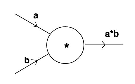
Before understanding backpropagation,let us go through the basic case on which majority of this post will be based. It consists of a node accepting two inputs a,b and producing an output. It will be referred to as default case for rest of this post.

The node accepts two inputs a,b and does a product operation on them and gives a*b as output.

Aim-Our aim is to increase the output by tweaking values of a and b.

Method#1

The first method is the most obvious one.Let us randomly increase the values of a and b by a small quantity h times a random number:

def product(a,b):
	return a*b
a=4
b=3
h=0.01
a=a+h*(random.random())
b=b+h*(random.random())
print(product(a,b))

The output for above program is 12.042 which is greater than 12 as was our aim.Although our aim is achieved but there are problems:

• This is a good strategy for small problems with few nodes but with millions of inputs and thousands of nodes which is easily possible in modern day networks this strategy of exhaustive search would be too time consuming.

• This is an unreliable method to increase value of the function.When we randomly increase the values of a and b,it might result in decrease in value of function.Have a look at the code below:

  def product(a,b):
  	return a*b
  a=-4
  b=-3
  h=0.01
  a=a+h*(random.random())
  b=b+h*(random.random())
  print(product(a,b))
  

The above code produces output 11.94 which is less than 12.The only difference was in initial values of a and b.Thus randomly increasing the values of a and b won’t suffice our aim.

Thus we can conclude that:

• We need more control over increasing the values of input.Essentially it means that there should be more controlled coefficient of h.
• The coefficient of h should be function of input or inputs as changing the initial values of input changed the behaviour of output.

Method#2

This control that we desire in the coefficient of h is given by derivative.Derivative of a function with respect to a variable is a pretty easy and straightforward concept.Let us understand by modifying our default case-

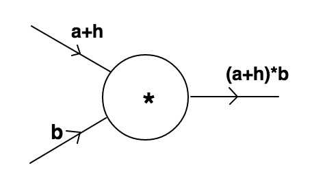
Let us increase the value of a by a small quantity h(same as in method 1) and let us give a name to our product function say f(a,b).Thus:

The new output can be calculated easily as (a+h)*b which can be expanded as a*b+h*b.Thus the output increases by a value of h*b as compared to default case.We can say that with increase of h in a the output increases by h*b,thus with a unit increase in a the output would have increased by b.This normalised effect of increase in value of one of the input on output is expressed as derivative of output with respect to that input.Note that when we take out derivative of function with respect to a variable then all other variables are kept constant. The mathematical interpretation of the derivative of function f with respect to a is defined as-

Similarly,the derivative of function f with respect to b can be found by increasing b by a small quantity h and normalising the difference between the final output(a*b+a*h) and initial output(a*b) that gives us a.

This is the numeric method of finding gradients.It has a significant drawback.Although it is less error prone but it takes lot of time to calculate derivatives this way.Time to introduce a new method of finding derivatives:Analytical method.

Method#3

Analytical gradient method:In order to calculate gradient using analytical gradient method we need to remember few basic rules of calculus(Refer Derivative-rules).These rules are derived from the numerical gradient method and are committed to memory so that they can be used directly.This saves us the computation time and space required for calculating derivatives.For f=a*b,the following can be directly stated-

def product(a,b):
	return a*b
a=-4
b=-3
h=0.01
a=a+h*b
b=b+h*a
print(product(a,b))

The output of above code is 12.252 which is greater than 12 as was our aim.

Why does this approach work?

To appreciate the beauty of derivative in updates of inputs a and b we have to dive into geometrical interpretation of derivative.Geometrically,derivative of a function with respect to a variable tells us the rate at which that function changes with respect to that variable.While reading ahead keep in mind those update rules given by-

Let us understand the effect of derivative in update rules in a single-variable system to get an intuition of what is happenning-

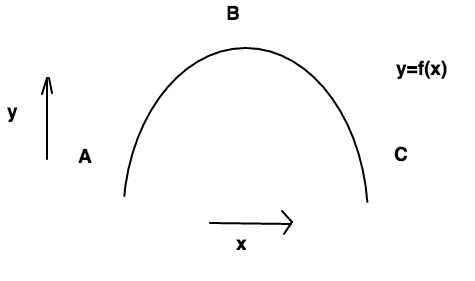
Above figure represents a function in single variable x.As x increases(from left to right) the function increases till point B and then decreases as we furthur increase x.Let us imagine two cases-

Case#1

Imagine we are at point A as shown in figure and we want to change the value of x in such a way that the value of funcion increases.From the figure it is clear that if we increase the value of x,the value of function increases.Now let us take a look at our update rule and see how it comes to this conclusion-

We know that our h>0 so whether x increases or decreases depends upon derivative of function with respect to x.Recall that derivative is nothing but the rate of change of function.At point A we can see that the function increases as x increases so the rate of change of function with respect to x at A is positive.This means that at point A the derivative of function with respect to x is positive.A positive derivative will make x increase through the update rule.

Case#2

Imagine that we are at point C as shown in figure.Everything remains same as case#1 but now we can see from figure that the value of function increases with decrease in value of x.At this time the derivative of funcion with respect to x will be negative as value of function decreases as x increases(i.e. the rate of change of function with x is negative).When we put a negative derivative in our update rule the value of x decreases as expected.

Thus the derivative captures the nature of our function and gives our update rule a sense of direction to obtain a higher value.

Case#3

Imagine that we are somewhere pretty close to point B(say we are on the left of it but pretty close to it).The value of derivative will be positive and the update rule would want to increase the value of xin order to increase the value of the function.But a condition could arise when value of h (stepsize) is sufficiently large that it overshoots the point B and thus decreasing the value of our function.Then we would have to adjust value of our stepsize(make it small of course!) in order to increase value of our function.Thus this approach of increasing value of inputs in direction of derivative would give us desired result for almost all functions you would encounter.(It fails for some poorly defined convex functions, but for now you do not need to worry about them.)

I will stop this post here.I hope that this post helped you develop an intuition about derivatives and their involvement in update rule.In the next post we will apply these principals in nested nodes and will finally see backpropagation.

Posted on 12 January,2017