Getting started with Tensorflow
It has been almost a year since Tensorflow was released by Google.Although there are a lot of deep learning libraries available(like Theano etc.) but Tensorflow is pretty big!One of the prominent reason is being backed by the big fish,Google! Also tensorflow has pretty great support for distributed systems.Considering the open-source popularity of tensorflow and recent advancements in neural network research,this library is here to stay.
In this post we will not only introduce tensorflow but also take a under-the-hood trip to its working.We will start off by going through basics of using tensorflow and analyze “computational graphs” that form the basis of tensorflow’s working.Later we will build a linear regression model that would further clarify its working.
Lets get started!!!
When we come across the name “Tensorflow”,the first thing that invariably comes to mind is the word “tensor”.Why “tensor”flow?What is a “tensor”?Well,not dwelling too much on its mathematical representation,consider tensor as a multidimensional array of numbers.Thus all scalars,vectors,matrices fall under the category of tensors. Let us try to add two tensors in tensorflow-
#import tensorflow
import tensorflow as tf
#declare constants
a=tf.constant(2,name="a")
b=tf.constant(3,name"b")
c=tf.add(a,b,name="c")
In above program the function tf.constant(value) is used to declare a constant of value value and tf.add(a,b) is used to add two tensors a and b. Let us now try to print the value of c:
#import tensorflow
import tensorflow as tf
#declare constants
a=tf.constant(2,name="a")
b=tf.constant(3,name="b")
c=tf.add(a,b,name="c")
print(c)
Output-
Tensor("Add:0", shape=(), dtype=int32)
Instead of a scalar tensor valued 5,the above program prints a weird tensor object.Why does this happen?Well,at first it might seem that the operations that we do in tensorflow are direct operations on multidimensional arrays but the truth is drastically different.This difference is actually the essence of tensorflow! When we do computations in tensorflow,instead of running them directly,tensorflow constructs a “computation graph”.
Computation Graph
Computation graph in tensorflow can be considered as network of nodes,with each node representing an operation.From generation of constant tensors to mathematical operations on them,all are represented in form of nodes and are referred to as ops.For our example of adding two constant tensors the computational graph can be visualized as:
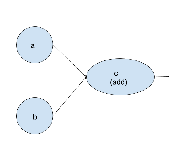 One of the important aspect of computation graph is that it does not has any numerical value until it is explicitly evaluated or run.Thus when we printed the value of
 c above it returned a tensor object rather than returning the numerical value of added tensors.
So the next logical question is “how do we run this computation graph?”.
In order to run a computation graph in tensorflow,a context is required.This context is encapsulated by a Session object.To clarify this concept,have a look at the code below:
#import tensorflow
import tensorflow as tf
#declare constants
a=tf.constant(2,name="a")
b=tf.constant(3,name="b")
c=tf.add(a,b,name="c")
#create a session
with tf.Session() as sess:
    #running the computation in session
    print(sess.run(c))
Output-
5
A Session object is created by the method tf.Session().The computation c in our computation graph would run in this session by calling the sess.run(c) method.The addition computation runs in our Session sess and yields a value of 5.
To avoid of passing the computation from the run method of our session object,tensorflow has concept of Interactive Session.Once an InteractiveSession object is created,a computation can be evaluated by calling the eval() method on it(instead of previously passing the computation from run method of Session object).This comes in handy when dealing with Ipython notebooks and other interactive environments.Have a look at the implementation below:
#import tensorflow
import tensorflow as tf
#declare constants
a=tf.constant(2,name="a")
b=tf.constant(3,name="b")
c=tf.add(a,b,name="c")
#create an Interactive session
sess=tf.InteractiveSession()
#just call eval() on the computation to be evaluated.
print(c.eval())
Output-
5
Why does the concept of computation graph exist?
One of the question that inevitably comes to mind while going through computation graph is the reason for existence of such system.Why can’t tensorflow do the computations directly on memory? Machine learning libraries like tensorflow are needed to do large numerical computations efficiently.These computations are not optimised in python and need to be carried out in a well optimised language outside python.Thus, there can be a lot of overhead from switching back to Python after every computation. This overhead is especially bad if you want to run computations on GPUs or in a distributed manner, where there can be a high cost to transferring data. TensorFlow also does its heavy lifting outside Python, but it takes things a step further to avoid this overhead. Instead of running a single expensive operation independently from Python, TensorFlow lets us describe a graph of interacting operations that run entirely outside Python. This approach is similar to that used in Theano or Torch.
Tensorflow Variables
The tensors that we have dealt with till now were constants.Tensorflow also has the concept of Variables. Any machine learning problem will inevitably involve some parameters that would need to be updated in order to optimize a function.These updatable parameters will be expressed in form of tensorflow variables. One basic difference between constant tensors and variable tensors is that the variable tensors need to be initialized explicitly unlike constant tensors.Have a look at the implementation below:
#import tensorflow
import tensorflow as tf
#add a constant tensor to our graph
W1=tf.ones((2,2))
#add a variable to our graph
W2=tf.Variable(tf.zeros((2,2)))
#make a session object
with tf.Session() as sess:
	#run the constant op
    print(sess.run(W1))
    #initialize all variables in our graph
    sess.run(tf.global_variables_initializer())
    #run the variable op
    print(sess.run(W2))
Output-
[[ 1.  1.]
 [ 1.  1.]]
[[ 0.  0.]
 [ 0.  0.]]
The function tf.global_variables_initializer() explicitly initializes all the variables tensors.The absence of this function will lead to generation of error in presence of Variables.
Placeholders and Feed dictionaries
Till now we have seen simple variable tensors and constant tensors in tensorflow.A class of operations called placeholder also exists to facilitate the input of data to the our computation graph.They act as dummy nodes that provide entry points for data to our graph. It is important to note that placeholder ops should be provided data at the time of execution of our computation graph.This task is accomplished with the help of feed dictionaries.Thus feed dictionaries act as an intermediate between our data and placeholder ops.On the other hand the placeholder ops transfer the data that they receive from feed dictionaries at the time of execution to our computation graph.To get the idea of syntax,have a look at the code below:
#import tensorflow
import tensorflow as tf
#add a placeholder to our graph
input1=tf.placeholder(tf.float32)
#add another placeholder to our graph
input2=tf.placeholder(tf.float32)
#add an addition op to our graph
output=tf.add(input1,input2)
#create a session object
with tf.Session() as sess:
    #run the output op by providing data to placeholders through feed dictionaries
    print(sess.run(output,feed_dict={input1:[3.],input2:[2.]}))
Output-
[ 5.]
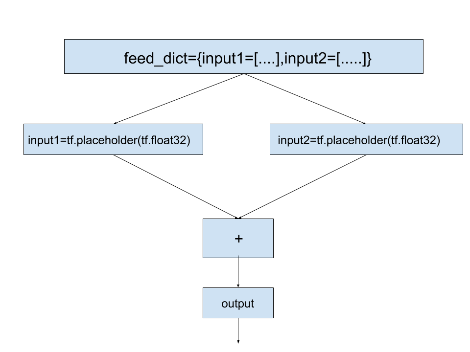
The above code is heavily commented and self explanatory.One of the noticable modification is inclusion of the argument feed_dict in the run() methos of our session object. Note that above code is just to give you a syntactical and logical feeling about placeholders and feed dictionaries.We will use this concept at scale when we implement linear regression model in tensorflow.To clarify further,the flow of data from feed_dict to placeholders can be graphically represented as:
Now that we have some idea of how computations take place in tensorflow,it is now a good time to implement a real model in tensorflow and analyze its working hands-on.Let us implement simple linear regression in tensorflow and string together all that we have learnt in this post.
Linear Regression in tensorflow
The problem of linear regression is arguably the simplest machine learning problem.Simply put,in a 2-dimensional context,given a set of points(data),we need to find a straight line that fits that data the best.We will implement this model by breaking it down in steps and using concepts that we have learnt so far in this post.
First things first,we need a dataset to implement regression on.Let us generate some random data as-
#importing tensorflow
import tensorflow as tf
#importing numpy
import numpy as np
#importing matplotlib for plots
import matplotlib.pyplot as plt
#x coordinate of data
X_data=np.arange(0,100,0.1)
#y coordinate of data
Y_data=X_data+20*np.sin(X_data/10)
#plotting the data
plt.scatter(X_data,Y_data)
plt.show()
Above code is pretty straightforward.To generate data we add some sinosoidal noise to the y coordinate.This give us the following plot:
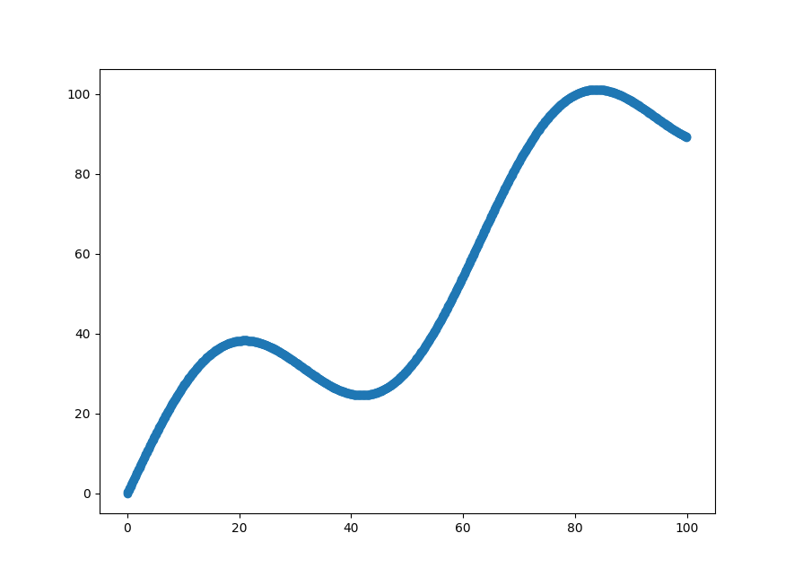
Our task is to fit a best possible straight line through this dataset.
Now that we have our input data,we need to process it so that we can transfer it to our model.We have 1000 data-points of both X_data and Y_data. Let us convert this data in form of 1000X1 tensors as-
#total data points
n_samples=1000
#X_data in form of 1000X1 tensor
X_data=np.reshape(X_data,(n_samples,1))
#Y_data in form of 1000X1 tensor
Y_data=np.reshape(Y_data,(n_samples,1))
Now that we have our data processed,we need to declare placeholders which would act as entry point of data to our computation graph.Here we will not transfer all of our 1000 datapoints at once to our computation graph.Rather we will do this in batches of size 100.
#batch size
batch_size=100
#placeholder for X_data
X=tf.placeholder(tf.float32,shape=(batch_size,1))
#placeholder for Y_data
Y=tf.placeholder(tf.float32,shape=(batch_size,1))
We have our placeholders ready.As we want to fit our data in a straight line,we need to dwell upon the variables that would be learnt in order to accomplish this task.We need to create a weight variable and a bias variable to generate predictions from our input data X.These predictions will be modified by updating weight and bias variables.Our aim would be to get our predictions as close as possible to Y.This effect would be captured by minimizing our root mean square error loss function.
#defining weight variable
W=tf.Variable(tf.random_normal((1,1)),name="weights")
#defining bias variable
b=tf.Variable(tf.random_normal((1,)),name="bias")
#generating predictions
y_pred=tf.matmul(X,W)+b
#RMSE loss function
loss=tf.reduce_sum(((Y-y_pred)**2)/n_samples)
To get the minimum value of this loss function we need to vary the values of weights and bias.This minimization is achieved using gradient-descent(refer here) which is implemented directly in tensorflow as follows:
#defining optimizer
opt_operation=tf.trainAdamOptimizer().minimize(loss)
#creating a session object
with tf.Session() as sess:
    #initializing the variables
    sess.run(tf.global_variables_initializer())
    #gradient descent loop for 500 steps
    for iteration in range(500):
      #selecting batches randomly
      indices=np.random.choice(n_samples,batch_size)
      X_batch,Y_batch=X_data[indices],Y_data[indices]
      #running gradient descent step
      _,loss_value=sess.run([opt_operation,loss],feed_dict={X:X_batch,y:Y_batch})
Above we define a optimization operation using the tf.trainAdamOptimizer()function which is a modified form of gradient descent algorithm.We also randomly select the batches of input data of batch size 100 and run our optimization operation.The for loop running 500 times during the training can be seen as 500 iterations in the gradient descent algorithm.After each iteration the values of weights and bias are updated.Each iteration randomly selects 100(batch_size) data points from the set of 1000(n_samples) and feeds it to the placeholders using feed dictionaries.
When we plot the straight line generated along with our initial dataset we see the following:
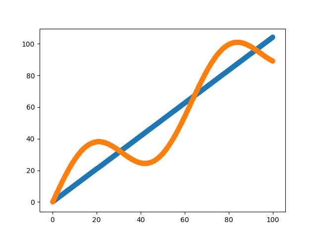 Thus we can see that we have obtained a pretty good linear fit to our curve.For the sake of completeness here is the full code:
import tensorflow as tf
import numpy as np
import matplotlib.pyplot as plt
#generating data
X_data=np.arange(0,100,0.1)
Y_data=X_data+20*np.sin(X_data/10)
#plotting the data
plt.scatter(X_data,Y_data)
#Uncomment below to see the plot of input data.
#plt.show()
n_samples=1000
X_data=np.reshape(X_data,(n_samples,1))
Y_data=np.reshape(Y_data,(n_samples,1))
#batch size
batch_size=100
#placeholder for X_data
X=tf.placeholder(tf.float32,shape=(batch_size,1))
#placeholder for Y_data
Y=tf.placeholder(tf.float32,shape=(batch_size,1))
#placeholder for checking the validity of our model after training
X_check=tf.placeholder(tf.float32,shape=(n_samples,1))

#defining weight variable
W=tf.Variable(tf.random_normal((1,1)),name="weights")
#defining bias variable
b=tf.Variable(tf.random_normal((1,)),name="bias")
#generating predictions
y_pred=tf.matmul(X,W)+b
#RMSE loss function
loss=tf.reduce_sum(((Y-y_pred)**2)/batch_size)
#defining optimizer
opt_operation=tf.train.AdamOptimizer(.0001).minimize(loss)
#creating a session object
with tf.Session() as sess:
    #initializing the variables
    sess.run(tf.global_variables_initializer())
    #gradient descent loop for 500 steps
    for iteration in range(5000):
        #selecting batches randomly
        indices=np.random.choice(n_samples,batch_size)
        X_batch,Y_batch=X_data[indices],Y_data[indices]
        #running gradient descent step
        _,loss_value=sess.run([opt_operation,loss],feed_dict={X:X_batch,Y:Y_batch})

    #plotting the predictions
    y_check=tf.matmul(X_check,W)+b
    pred=sess.run(y_check,feed_dict={X_check:X_data})
    plt.scatter(X_data,pred)
    plt.scatter(X_data,Y_data)
    plt.show()
So this was our implementation of linear regression model in tensorflow.In the next post we will try to extend our knowledge of tensorflow by building a different model.It would be fun!Stay tuned!
Posted on 26 January,2017