Neural Stacks-An Explanation

Recently I stumbled upon this paper by Google Deepmind titled “Learning to transduce with unbounded memory”.I think it will be pretty fascinating to implement this paper.The implementation will be based on neural stacks accomplishing the sequence reversal task.We will first implement scaled down version of neural stacks using python and numpy and then look to implement it in tensorflow.As I would be implementing and posting subsequently as I get time,this section of blog may be updated less frequently(still pretty frequently!).There may be some mistakes in implementations and I may have to disregard my previous implementations to correct those mistakes. I suggest you to follow this portion of blog with open mind as I will post here open to suggestions and criticism.

In this post I will first draw an outline of the task of sequence reversal using the neural stack.Then we will look at the design of neural stack and would implement the forward propagation through the stack.

Lets get started!!!

Outline

We know that Recurrent neural networks(RNNs) can use hidden layers as memory to process arbitrary sequences of inputs.But as the length of input sequence increase,the hidden layers have to increase in order to capture long term dependencies.This makes the net deeper.A deeper net should work well(at least in theory) but that is not the case.Various problems such as exploding and dying gradients,increase in number of parameters due to deeper nets etc. make the learning difficult and inefficient. To counter these difficulties,LSTM(Long short term memory) cells were introduced.Although they work really well as compared to vanilla RNNs,still they fail to generalize for longer strings in context of transduction tasks like sequence reversal etc. The main problem,according to me,this paper wants to tackle is of generalization of transduction tasks for larger strings as compared to the training data(because larger strings would require larger computational resources during training).The paper does this by introducing an extensible memory which is logically unbounded(i.e. infinite capacity in theory but definitely would be limited due to machine constraints).This memory structure(e.g. a neural stack) is controlled with the help of a Recurrent neural network.The benefit that we get from such arrangement is we get logically unbounded memory for our network which is independent from the parameter and nature of our RNN(unlike previously when we had to increase the depth of network to increase the memory capacity of our network).

I hope this outline gave you an idea of what the author wants to achieve with this paper.According to me,during analysis of any research paper,outline is the most important tool.It gives us an idea of what is coming and also aligns our direction of thinking to that of the author’s.

What is a Stack?

Neural stack is inspired from one of the traditional data structure “Stack”.A stack is a linear data structure that works on the principle of LIFO(Last-in-first-out).Just imagine a stack of books.You would stack them up one over another and at the time of retrival you will pick a book from top of the stack i.e. the one that was stacked last(in) would be retrived(out) first. The act of stacking up objects(here books or else numbers!) is called “push” operation while the act of retrieval is called “pop” operation.Another operation is possible in which we can read the object on top of the stack.This is called “peek/read” operation.For this paper,we will use the “read” term. Thus it is pretty straightforward to reverse a sequence using a traditional stack.Just push the string that we want to reverse into the stack(character-by-character/number-by-number you get that!) and just pop those entities out.Refer the figure: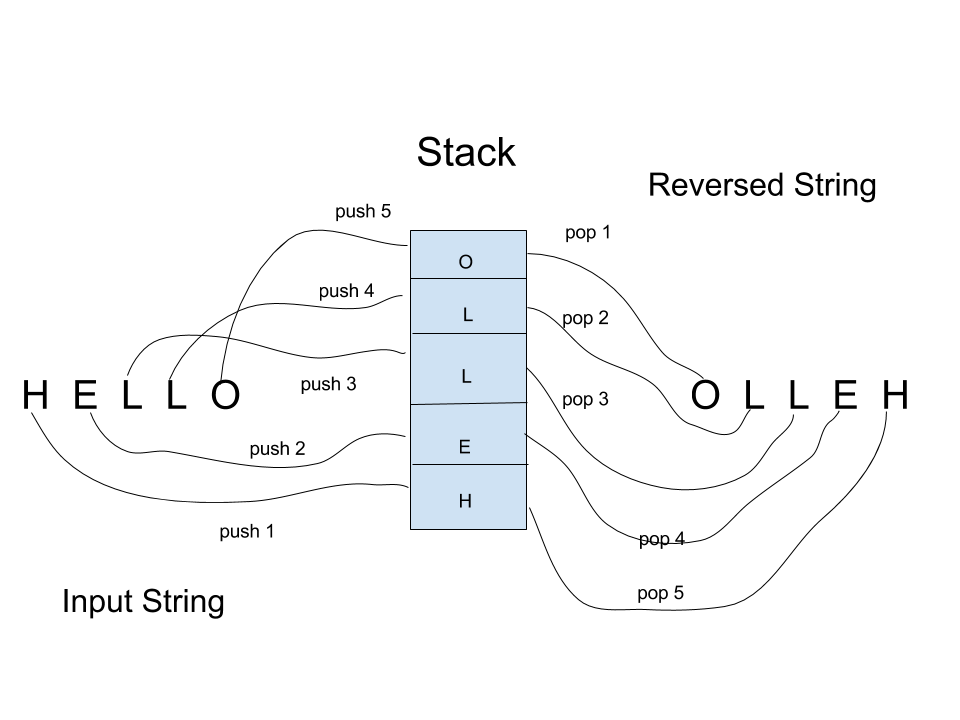 stack

Neural Stack

Traditional stacks are fine but if we want to connect a stack with a recurrent network or in fact any network then it should be differentiable.Networks learn using backpropagation and for backpropagation of error every part of our network should be differentiable.Thus the mantra is

“If it is differentiable,it is trainable”

As our stack will be connected to a RNN,it should be differentiable as well.In order to render these stacks differentiable,the paper comes up with rendering the discrete operations push and pop continuous by representing them with a value in interval (0,1) which represent the degree of certainity with which the controller(RNN) wishes to push a vector \(\Large\mathcal{v}\) onto the stack or pop the top of the stack.

Implementation of Neural Stack-

The author implements the neural stacks by using a value matrix \(\Large{V}\) which acts as a expandable stack for storing the vectors as they are pushed.Each vector in the value matrix has a strength value which is stored in another vector called strength vector \(\Large{s}\).The strength values of vectors in value matrix can be seen as certainty by which the vector is in the value matrix.A zero strength value would signify the absence of corresponding vector from the value matrix. Both strength vector and value matrix expand with time as new values are pushed into the value matrix.

The implementation of neural stack is based on three key formulas.I will explain the significance of these formulas and their respective python implementation.

The first formula gives description of our value matrix:

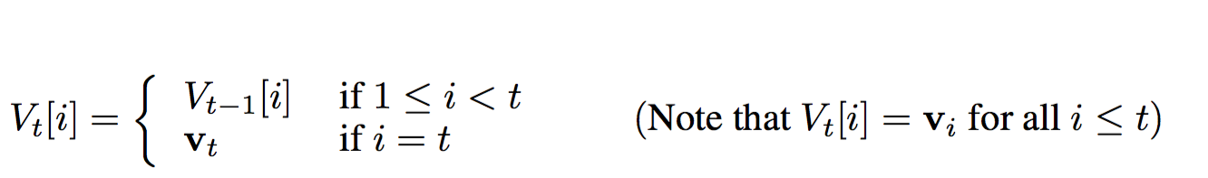
The above formula represents the effect of push operation on our value matrix,\(\Large{V_t}\).Assuming on every time step we push into our value matrix,the index \(\Large{i}\) represents the \(\Large{i^{th}}\) entry in our value matrix. Thus at any time instant \(\Large{t}\),our value matrix would be comprised of all the vectors pushed until time \(\Large{t}\) and the vector pushed at the time \(\Large{t}\) i.e. \(\Large{v_{t}}\). One of the important things to take note here is that,once a vector is added to our value matrix,it is never modified.For modifications during pop operations we modify strength vector rather than vectors in our value matrix.

The second formula describes our strength vector:

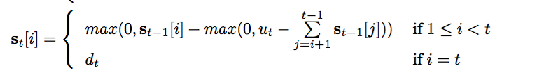
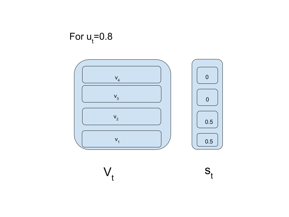
The above formula represents the effect of push and pop operations on our strength vector. \(\Large{u_t}\) is the pop signal and \(\Large{d_t}\) is the push signal.Both the value lie in the range (0,1).\(\Large{s_t}\) denotes the strength vector at time \(\Large{t}\) while \(\Large{s_{t-1}}\) is the strength vector at time \(\Large{t-1}\). When we receive a pop signal(\(\Large{u_t}\)), we traverse down the strength vector from highest index to lowest index repeatedly subtracting the scalars of \(\Large{s_{t-1}}\) from \(\Large{u_t}\).If \(\Large{u_{t}}\) is greater than the next scalar then that scalar is set to zero(of course after subtraction!) and the traversal continues.If \(\Large{u_t}\) is less than the next scalar then \(\Large{u_t}\) is subtracted from that scalar and traversal stops. When we receive a push signal(\(\Large{d_t}\)),the \(\Large{t^ {th}}\) entry of the strength vector is modified as \(\Large{d_t}\). When push and pop signals are received first pop takes place which is followed by push. 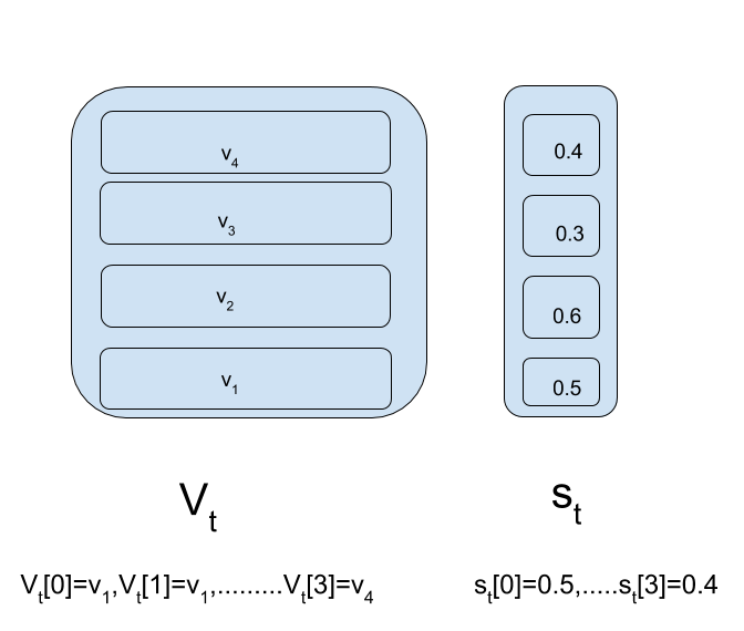Have a look at figures below to clarify notations and pop operation:The first figure will be referred to as “reference-figure”. pop

This process of modification of strength vector can be represented in python as:

#initializing strength dictionary
strength={}
def strength_time(time,push_certainity,pop_certainity):

    for var in reversed(range(time)):
        if strength[var]< pop_certainity:
            pop_certainity-=strength[var]
            strength[var] = 0
        else:
            strength[var]-=pop_certainity
            pop_certainity = 0
            break
    strength[time] = push_certainity

The third formula describes the read operation

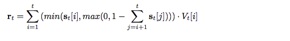
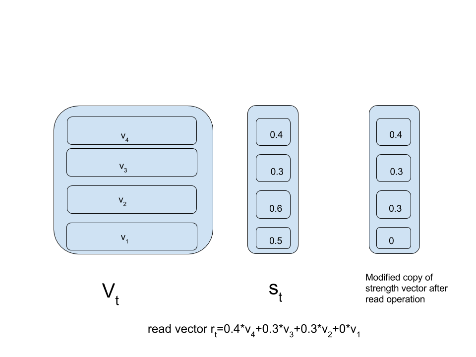
The above formula represents the read vector.While reading from our stack,we set a fixed initial read quantity of 1.A temporary copy of strength vector is made.Similar to pop operation,the copy of strength vector is traversed from highest index to lowest.If the next scalar is less than the read value then its value is preserved and is subtracted from the read quantity.If the next scalar is more than read value then its value is made equal to remaining read quantity and rest all scalars are set to zero.This resulting copy of strength values is then multiplied with corresponding vectors in value matrix and by adding these product values read vector is generated. Have a look at figure below to make things clearer: read

Implementing this in python we get:

def read_time(time):
    #returns read vector at time 'time'
    #initial read value of 1
    read=1
    read_vector=np.zeros(input_size)
    #duplicate of strenth vector to modify it at time of read operation
    temp_strength=copy.deepcopy(strength)
    #traversing through strength vector from top
    for var in reversed(range(time+1)):
        if temp_strength[var]< read:
            read-=temp_strength[var]
        else:
            temp_strength[var]=read
            unwanted=set(temp_strength.keys())-set(range(var,time+1))
            for keys in unwanted:
                temp_strength[keys]=0
            break
    for var in Value.keys():
        read_vector+=(temp_strength[var]*Value[var])
    return read_vector

Checking our implementation: Below code is consistent with our read figure.Four vectors are pushed into our value matrix with the help of pushPop function.


import numpy as np
import copy
Value={}
strength={}
input_size=4

value_1=np.zeros(input_size)
value_1[0]=1        #[1 0 0 0]
value_2=np.zeros(input_size)
value_2[1]=1        #[0 1 0 0]
value_3=np.zeros(input_size)
value_3[2]=1        #[0 0 1 0]
value_4=np.zeros(input_size)
value_4[3]=1        #[0 0 0 1]



def read_time(time):
    #returns read vector at time 'time'
    #initial read value of 1
    read=1
    read_vector=np.zeros(input_size)
    #duplicate of strenth vector to modify it at time of read operation
    temp_strength=copy.deepcopy(strength)
    #traversing through strength vector from top
    for var in reversed(range(time+1)):
        if temp_strength[var]< read:
            read-=temp_strength[var]
        else:
            temp_strength[var]=read
            unwanted=set(temp_strength.keys())-set(range(var,time+1))
            for keys in unwanted:
                temp_strength[keys]=0
            break
    for var in Value.keys():
        read_vector+=(temp_strength[var]*Value[var])
    return read_vector



def strength_time(time,push_certainity,pop_certainity):

    for var in reversed(range(time)):
        if strength[var] < pop_certainity:
            pop_certainity-=strength[var]
            strength[var] = 0
        else:
            strength[var]-=pop_certainity
            pop_certainity = 0
            break
    strength[time] = push_certainity
    print(strength)


def pushPop(push_value,push_certainity,pop_certainity,time):

    strength_time(time,push_certainity,pop_certainity)
    Value[time]=push_value
    return read_time(time)

pushPop(value_1,0.5,0,0)
pushPop(value_2,0.6,0,1)
pushPop(value_3,0.3,0,2)
print(pushPop(value_4,0.4,0,3)) #prints [0 .3 .3 .4]

Above program outputs [0 .3 .3 .4] which is consistent with 0.4*v4+0.3*v3+0.3*v2+0*v1.

In the next post we will look to implement backpropagation through our neural stack.

Posted on 22 January,2017